Recently I went through a post describing how one can use Bayesian Data Analysis tools to answer questions like How long does it take for one to respond to message on Google Hangout ? I was intrigued and wanted to see if I could find out my response time ? Since Skype is our preferred choice of communication in office, so I decided to replicate the whole process for it.
Data Preparation
Skype maintains a local database of all of our conversations. On a linux machine you can find the main.db file in ~\.Skype\<your_username>\ folder. This database contains multiple tables, but we will only be working with the messages table.
We will be working with only following attributes
| Field | Description |
|---|---|
| convo_id | Conversation Id |
| author | Sender of the message |
| timestamp | Timestamp |
Feature Engineering
Since we are trying to find out how much time does it take for me to respond to messages, it would be good if we could create features related to timestamp.
- We will create feature called prev_timestamp which would represent the timestamp of the previous message, similarly we will create a feature called prev_author which would store the sender of the previous message.
- We will then calculate the delay in response both in seconds and minutes
- Decompose the timestamp to find out day of the week, both year and month and whether it was a weekend or not.
Plot that describe my typical response times
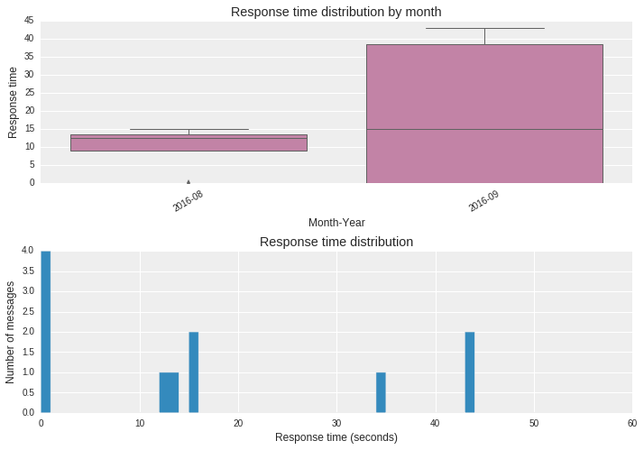
These plots give a monthly and overall perspective of my response times.
Bayesian Data Analysis ?
Let’s try to understand what Bayesian analysis is all about by using the following example
A curious boy watches the number of cars that pass by his house every day. He diligently notes down the total count of cars that pass per day. Over the past week, his notebook contains the following counts: 12, 33, 20, 29, 20, 30, 18
From a Bayesian’s perspective, this data is generated by a random process. However, now that the data is observed, it is fixed and does not change. This random process has some model parameters that are fixed. However, the Bayesian uses probability distributions to represent his/her uncertainty in these parameters. This thinking resonates with the Bayes formula that most of us are familiar with
p(theta | data) = (p(data | theta) * p(theta)) / p(data)
where p(theta | data) = posterior, p(data | theta) = likelihood, p(theta) = prior, p(data) = marginal likelihood
Bayesian line of thinking can be summarized as:
- We observe counts of data (y) for each observation i ( Observed Data )
- This data was generated by a random process which we believe can be represented as a negative binomial distribution ( Likelihood )
- Negative binomial distribution has two parameters (alpha and mu) which enables it to vary its variance independently of its mean.
- We will model mu as a uniform distribution and alpha as a exponential distribution because we do not have a opinion about their range.
Then we will draw many samples and use MCMC (Markov Chain Monte Carlo) sampling to find out areas with high probability. The MCMC sampler draws parameter values from the prior distribution and computes the likelihood that the observed data came from a distribution with these parameter values.
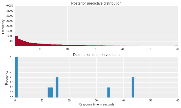
The above figure shows that our choice of distribution is correct and posterior predictive distribution matches with the distribution of the observed data.
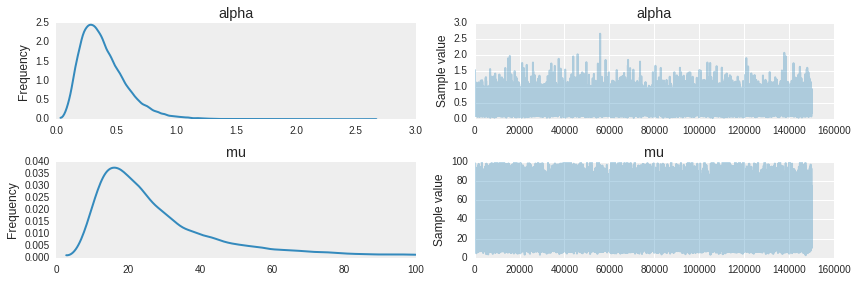
As you can see the distribution is pretty wide which represents our belief in the values and this is because there wasn’t sufficient data to work with, but what it says in effect is that if you would message me on Skype then you should expect a response from me within 20-40 seconds with greater degree of confidence.
If anyone wants to go through the whole process please find the link to notebook
In the next post we will try to answer some other interesting questions using the same dataset, so stay tuned.